$$ \newcommand{\initvar}{v_0^2} \newcommand{\cd}{\overset{d}{\to}} \newcommand{\var}{\text{var}} \newcommand{\cov}{\text{cov}} \newcommand{\argmax}[1]{\underset{#1}{\arg\max}} \newcommand{\argmin}[1]{\underset{#1}{\arg\min}} \newcommand{\iid}{\overset{\textrm{iid}}{\sim}} \newcommand{\indep}{\overset{\textrm{indep}}{\sim}} \newcommand{\tr}{{\scriptscriptstyle\mathsf{T}}} \newcommand{\com}{,\,} \newcommand{\given}{\,|\,} \newcommand{\acal}{\mathcal{A}} \newcommand{\bcal}{\mathcal{B}} \newcommand{\ccal}{\mathcal{C}} \newcommand{\dcal}{\mathcal{D}} \newcommand{\ecal}{\mathcal{E}} \newcommand{\fcal}{\mathcal{F}} \newcommand{\gcal}{\mathcal{G}} \newcommand{\hcal}{\mathcal{H}} \newcommand{\ical}{\mathcal{I}} \newcommand{\jcal}{\mathcal{J}} \newcommand{\kcal}{\mathcal{K}} \newcommand{\lcal}{\mathcal{L}} \newcommand{\mcal}{\mathcal{M}} \newcommand{\ncal}{\mathcal{N}} \newcommand{\ocal}{\mathcal{O}} \newcommand{\pcal}{\mathcal{P}} \newcommand{\qcal}{\mathcal{Q}} \newcommand{\rcal}{\mathcal{R}} \newcommand{\scal}{\mathcal{S}} \newcommand{\tcal}{\mathcal{T}} \newcommand{\ucal}{\mathcal{U}} \newcommand{\vcal}{\mathcal{V}} \newcommand{\wcal}{\mathcal{W}} \newcommand{\xcal}{\mathcal{X}} \newcommand{\ycal}{\mathcal{Y}} \newcommand{\zcal}{\mathcal{Z}} \newcommand{\EE}{\mathbb{E}} \newcommand{\NN}{\mathbb{N}} \newcommand{\PP}{\mathbb{P}} \newcommand{\QQ}{\mathbb{Q}} \newcommand{\RR}{\mathbb{R}} \newcommand{\ZZ}{\mathbb{Z}} \newcommand{\BA}{\mathbf{A}} \newcommand{\BB}{\mathbf{B}} \newcommand{\BC}{\mathbf{C}} \newcommand{\BD}{\mathbf{D}} \newcommand{\BE}{\mathbf{E}} \newcommand{\BF}{\mathbf{F}} \newcommand{\BG}{\mathbf{G}} \newcommand{\BH}{\mathbf{H}} \newcommand{\BI}{\mathbf{I}} \newcommand{\BJ}{\mathbf{J}} \newcommand{\BK}{\mathbf{K}} \newcommand{\BL}{\mathbf{L}} \newcommand{\BM}{\mathbf{M}} \newcommand{\BN}{\mathbf{N}} \newcommand{\BO}{\mathbf{O}} \newcommand{\BP}{\mathbf{P}} \newcommand{\BQ}{\mathbf{Q}} \newcommand{\BR}{\mathbf{R}} \newcommand{\BS}{\mathbf{S}} \newcommand{\BT}{\mathbf{T}} \newcommand{\BU}{\mathbf{U}} \newcommand{\BV}{\mathbf{V}} \newcommand{\BW}{\mathbf{W}} \newcommand{\BX}{\mathbf{X}} \newcommand{\BY}{\mathbf{Y}} \newcommand{\BZ}{\mathbf{Z}} \newcommand{\Ba}{\mathbf{a}} \newcommand{\Bb}{\mathbf{b}} \newcommand{\Bc}{\mathbf{c}} \newcommand{\Bd}{\mathbf{d}} \newcommand{\Be}{\mathbf{e}} \newcommand{\Bf}{\mathbf{f}} \newcommand{\Bg}{\mathbf{g}} \newcommand{\Bh}{\mathbf{h}} \newcommand{\Bi}{\mathbf{i}} \newcommand{\Bj}{\mathbf{j}} \newcommand{\Bk}{\mathbf{k}} \newcommand{\Bl}{\mathbf{l}} \newcommand{\Bm}{\mathbf{m}} \newcommand{\Bn}{\mathbf{n}} \newcommand{\Bo}{\mathbf{o}} \newcommand{\Bp}{\mathbf{p}} \newcommand{\Bq}{\mathbf{q}} \newcommand{\Br}{\mathbf{r}} \newcommand{\Bs}{\mathbf{s}} \newcommand{\Bt}{\mathbf{t}} \newcommand{\Bu}{\mathbf{u}} \newcommand{\Bv}{\mathbf{v}} \newcommand{\Bw}{\mathbf{w}} \newcommand{\Bx}{\mathbf{x}} \newcommand{\By}{\mathbf{y}} \newcommand{\Bz}{\mathbf{z}} \newcommand{\Balpha}{\boldsymbol{\alpha}} \newcommand{\Bmu}{\boldsymbol{\mu}} \newcommand{\Btheta}{\boldsymbol{\theta}} \newcommand{\Beta}{\boldsymbol{\eta}} \newcommand{\Bepsilon}{\boldsymbol{\varepsilon}} \newcommand{\Bbeta}{\boldsymbol{\beta}} \newcommand{\BLambda}{\boldsymbol{\Lambda}} \newcommand{\BSigma}{\boldsymbol{\Sigma}} \newcommand{\BOmega}{\boldsymbol{\Omega}} \newcommand{\BPsi}{\boldsymbol{\Psi}} \newcommand{\BGamma}{\boldsymbol{\Gamma}} \newcommand{\BPhi}{\boldsymbol{\Phi}} \newcommand{\Bphi}{\boldsymbol{\phi}} \newcommand{\BUpsilon}{\boldsymbol{\Upsilon}} \newcommand{\BXi}{\boldsymbol{\Xi}} \newcommand{\Bpi}{\boldsymbol{\pi}} \newcommand{\Bzero}{\mathbf{0}} \newcommand{\Bone}{\mathbf{1}} \newcommand{\N}{\text{N}} \newcommand{\dd}{\text{d}} $$

Time series potpourri

Ed Iversen and John Zito

Duke University
STA 440 Spring 2026

Recap

Time series models

  • A time series is a set of measurements collected over time;

  • We model these data as a sequence of dependent random variables:

\[ \mathbf{y}_{0:T} = \{\mathbf{y}_0,\,\mathbf{y}_1,\,\mathbf{y}_2,\,...,\,\mathbf{y}_T\}. \]

  • A time series model is “just” their joint probability distribution:

\[ p(\mathbf{y}_{0:T}) = p(\mathbf{y}_0)\prod_{t=1}^Tp(\mathbf{y}_t\,|\,\mathbf{y}_{0:t-1}). \]

The autoregression of order \(p\)

\[ \begin{aligned} y_t &= \beta_0 + \beta_1 y_{t-1} + \beta_2 y_{t-2} + \cdots + \beta_p y_{t-p} + \varepsilon_t, \quad \varepsilon_t\iid\text{N}(0\com\sigma^2). \end{aligned} \]

This implies a joint distribution written marginal-conditional style:

\[ \begin{aligned} p(y_{1:T}\mid y_0\com y_{-1}\com ...\com y_{1-p}) &= \prod_{t=1}^Tp(y_t\mid y_{1-p:t-1})\\ \\ &= \prod_{t=1}^Tp(y_t\mid y_{t-p:t-1}). \end{aligned} \]

The joint distribution is just a big ol’ multivariate normal with a structured mean and covariance that depend on the parameters.

Estimation

Similar to iid regression:

  • Classical approach: MLE = OLS;
  • Bayesian approach: normal-inverse-gamma conjugate prior.

But the inferential theory is very different!

Probabilistic prediction

To generate interval and density predictions \(h\)-steps-ahead:

  • Classical approach: bootstrap;
  • Bayesian approach: posterior predictive simulation.

These incorporate data and parameter estimation uncertainty.

Hyperparameter tuning

The lag order \(p\) is a hyperparameter that must be selected:

  • eyeball ACF plots;
  • optimize canned criteria like AIC or BIC;
  • time series cross validation.

The moving average model

Why?

We have seen this so far:

\[ y_t = \beta_0 + \sum\limits_{l=1}^p\beta_ly_{t-l} + \underbrace{ u_t }_{\text{iid}} . \]

What if there is time series dependence in the error term as well?

What kind?

Autoregressive moving average (ARMA)

ARMA(\(p\), \(q\)):

\[ y_t = \beta_0 + \underbrace{\sum\limits_{l=1}^p\beta_ly_{t-l}}_{\text{autoregressive}} + \underbrace{\sum_{i=1}^q\theta_i\varepsilon_{t-i}}_{\text{moving average}} + \varepsilon_t, \quad \varepsilon_t \iid \N(0\com \sigma^2) . \]

Flexible class of models that can capture pretty generic linear dependencies.

  • \(p=q=0\) gives the iid model;
  • \(q=0\) gives the pure AR(\(p\)) we’ve already seen;
  • \(p=0\) gives the pure MA(\(q\)), which is seldom used on its own.

What is the joint distribution?

It’s normal! The mean and covariance depend on the AR and MA parameters and the error variance:

\[ \begin{bmatrix} y_1 & y_2 & \cdots & y_T \end{bmatrix}^\tr \sim\N_T\left(\Bmu\com \BSigma\right). \]

Don’t worry about the details, but there are theorems that say the ARMA model is flexible enough to capture any stable, linear time series dependence if \(p\) and \(q\) are sufficiently large.

Graphical structure

Consider the ARMA(1, 1):

\[ y_t=\beta_0+\beta_1y_{t-1}+\theta_1\varepsilon_{t-1}+\varepsilon_t, \quad \varepsilon_t\iid\N(0\com \sigma^2). \]

Then:

\[ \begin{matrix} y_0 & \to & y_1 & \to & y_2 & \to & y_3 & \to & y_4 & \to &\cdots \\ & \nearrow & \uparrow & \nearrow & \uparrow & \nearrow & \uparrow & \nearrow & \uparrow & \nearrow & \\ \varepsilon_0 & & \varepsilon_1 & & \varepsilon_2 & & \varepsilon_3 & & \varepsilon_4 & & \\ \end{matrix} \]

Autocovariance

  • The moving average piece is always stable;
  • If the AR piece is stable as well, then we have a shift-invariant autocovariance function

\[ \gamma(h)=\cov(y_{t+h}\com y_{t}). \]

  • The formulas aren’t pretty, but a computer can handle it easily;
  • We know an AR(1) is stable if \(|\beta_1|<1\). For the general AR(p), it’s complicated.

ACF of the ARMA

#| '!! shinylive warning !!': |
#|   shinylive does not work in self-contained HTML documents.
#|   Please set `embed-resources: false` in your metadata.
#| standalone: true
#| viewerHeight: 700

library(shiny)

plot_arma_acf <- function(ar = numeric(), ma = numeric(), lag.max = 10){
  y_vals <- ARMAacf(ar = ar, ma = ma, lag.max = lag.max)
  plot(0:lag.max, y_vals, pch = 19, ylim = c(-1, 1),
       xlab = "h", ylab = expression(rho~"(h)"))
  segments(0:lag.max, 0, 0:lag.max, y_vals)
  abline(h = 0, col = "lightgrey")
}

# Define UI for application that draws a histogram
ui <- fluidPage(
  
  # Application title
  titlePanel("Theoretical autocorrelation of a stationary ARMA(2, 2)"),
  
  # Sidebar with a slider input for number of bins 
  sidebarLayout(
    sidebarPanel(
      sliderInput("b1",
                  "β₁",
                  min = -2,
                  max = 2,
                  value = 0,
                  step = 0.05),
      sliderInput("b2",
                  "β₂",
                  min = -2,
                  max = 2,
                  value = 0,
                  step = 0.05),
      sliderInput("th1",
                  "θ₁",
                  min = -0.99,
                  max = 0.99,
                  value = 0,
                  step = 0.01),
      sliderInput("th2",
                  "θ₂",
                  min = -0.99,
                  max = 0.99,
                  value = 0,
                  step = 0.01),
      sliderInput("H",
                  "H",
                  min = 0,
                  max = 50,
                  step = 1,
                  value = 20)
    ),
    
    # Show a plot of the generated distribution
    mainPanel(
            plotOutput("acf", height = "400px"),
      plotOutput("stationarityPlot", height = "400px"),
      verbatimTextOutput("stationarity")
    )
  )
)

# Define server logic required to draw a histogram
server <- function(input, output) {
  
  output$acf <- renderPlot({
    b1 <- input$b1
    b2 <- input$b2
    th1 <- input$th1
    th2 <- input$th2
    H <- input$H
    
    plot_arma_acf(ar = c(b1, b2), ma = c(th1, th2), lag.max = H)

  })
  
    output$stationarityPlot <- renderPlot({
    b1 <- input$b1
    b2 <- input$b2
    
    # triangle vertices
    tri_x <- c(2, -2, 0)
    tri_y <- c(-1, -1, 1)
    par(mar = c(4, 4, 0.1, 4))
    plot(tri_x, tri_y, type = "n",
         xlab = expression(beta[1]),
         ylab = expression(beta[2]),
         xlim = c(-2.1, 2.1),
         ylim = c(-1.1, 1.1),
         xaxt = "n", yaxt = "n", bty = "n")
    axis(1, at = c(-2, 0, 2), pos = 0)
    axis(2, at = c(-1, 0, 1), pos = 0)
    
    polygon(tri_x, tri_y, col = rgb(0, 0, 1, 0.2), border = "blue", lwd = 2)
    points(b1, b2, pch = 19, col = "red", cex = 1.5)
  })
}

# Run the application 
shinyApp(ui = ui, server = server)

Estimation

It’s a mess:

  • The maximum likelihood problem for ARMA must be solved numerically;
  • There is no conjugate prior, and MCMC is a bit of a nightmare here.

Base R ships with some basic tools.

Simulate an ARMA

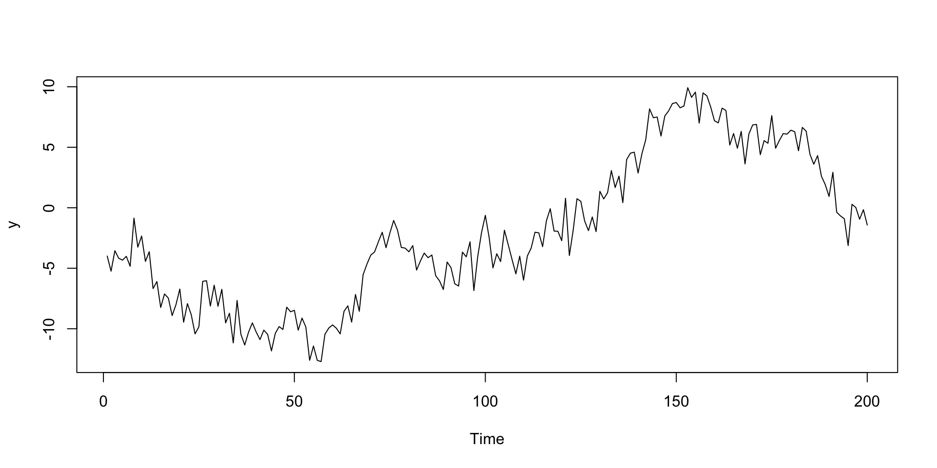
This is a function in base:

set.seed(8675309)

T <- 200
y <- arima.sim(n = T, model = list(ar = 0.99, ma = -0.4), sd = sqrt(2))

plot(y)

Fit an ARMA numerically

This is a function in base:

my_arma_fit <- arima(y, order = c(1, 0, 1))

my_arma_fit

Call:
arima(x = y, order = c(1, 0, 1))

Coefficients:
         ar1      ma1  intercept
      0.9871  -0.4307    -2.2742
s.e.  0.0089   0.0595     3.4451

sigma^2 estimated as 2.131:  log likelihood = -360.85,  aic = 729.69

Not far from the true values we provided. It’s tougher mathematically than iid regression, but we have asymptotic statistical theory for ARMA models (even when they’re not stable!).

Predict

This is a function in base:

H <- 30
fc <- predict(my_arma_fit, n.ahead = H)

head(fc$pred) # point prediction
Time Series:
Start = 201 
End = 206 
Frequency = 1 
[1] -1.000734 -1.017113 -1.033281 -1.049241 -1.064996 -1.080549
head(fc$se) # predictive standard error
Time Series:
Start = 201 
End = 206 
Frequency = 1 
[1] 1.459916 1.670697 1.853169 2.015144 2.161334 2.294846

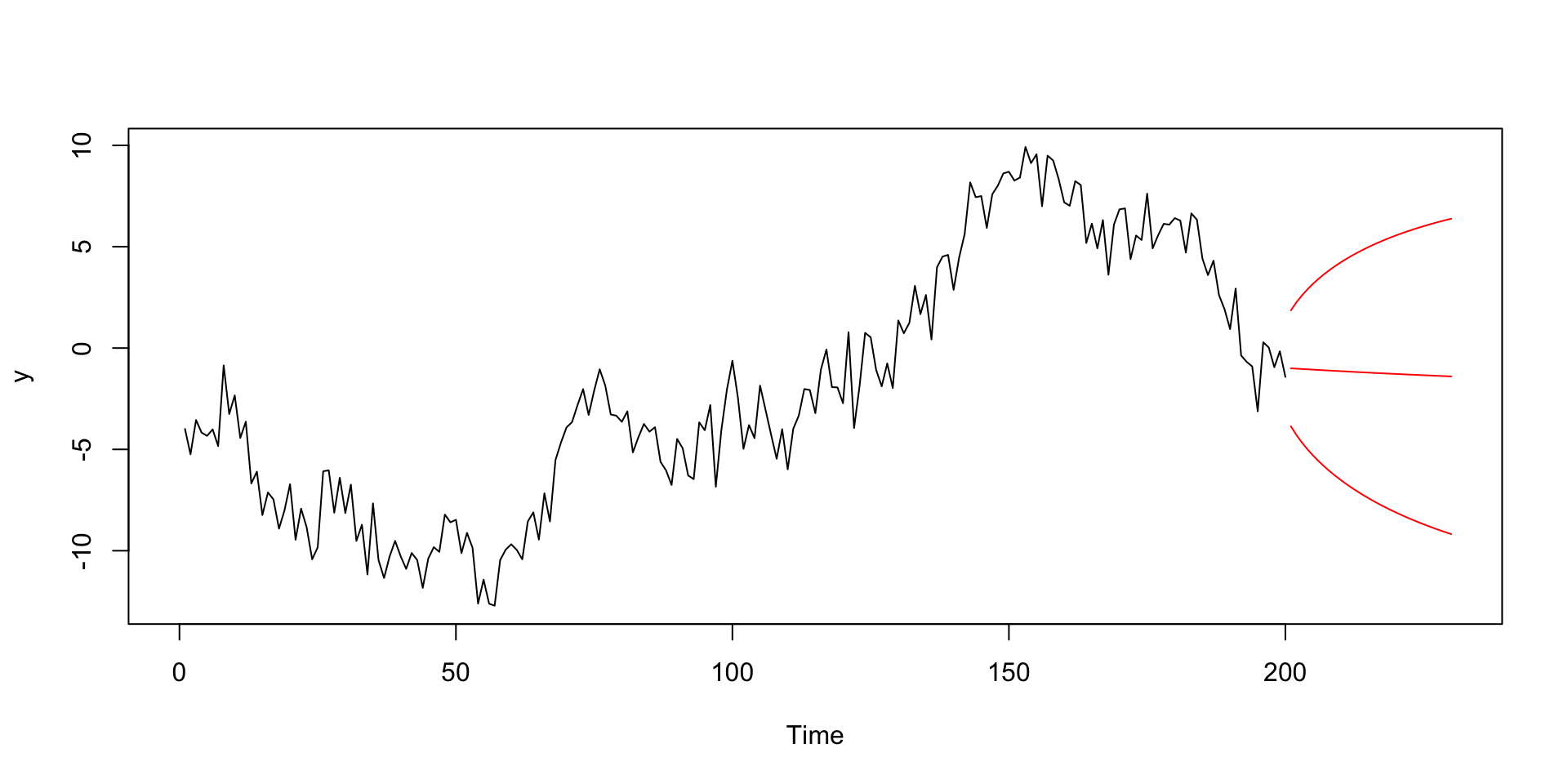
Poor man’s fan chart

plot(y, xlim = c(0, T + H))
lines(fc$pred, col = "red")
lines(fc$pred + 1.96 * fc$se, col = "red")
lines(fc$pred - 1.96 * fc$se, col = "red")

The hyndmanverse

  • Textbook is free online;
  • Very popular is some quarters;
  • Accompanying software is inspired by the tidyverse and very well-documented:
library(tsibble)
library(fable)

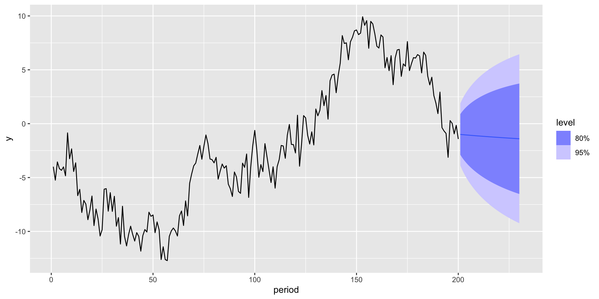
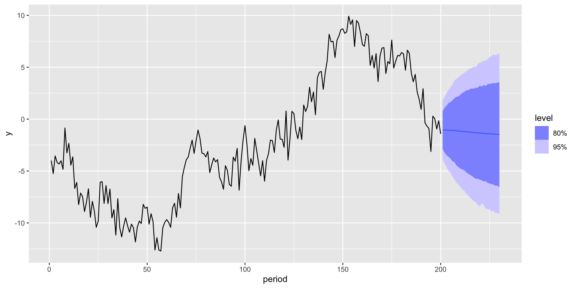
Only includes data uncertainty (no bootstrap!)

my_data = tsibble(period = 1:T, y = y, index = period)  

my_data |>
  model(my_model = ARIMA(y ~ 1 + pdq(1, 0, 1))) |>
  forecast(h = 30) |>
  autoplot(my_data)

Data and parameter estimation uncertainty

Not much difference because everything is cooked up nice here:

my_data |>
  model(my_model = ARIMA(y ~ 1 + pdq(1, 0, 1))) |>
  forecast(h = 30, bootstrap = TRUE, times = 5000) |>
  autoplot(my_data)

State space models

State space models (SSMs)

State space models are a meta-family of models that nest as special cases most time series models you will encounter in practice. SSMs are…

  • time series models;
  • graphical models;
  • latent variable models;
  • hierarchical models;
  • Bayesian models.

This makes them really rich and interesting! Anything you know about those separate areas of statistics helps with studying SSMs.

The main idea

  • State space models are first and foremost latent variable models;

  • They treat the observed time series \(\By_t\) as a noisy or corrupted version of an unobserved (or latent) time series \(\Bs_t\);

  • The goal of inference is to use what we observed (\(\By_t\)) to learn about what we didn’t observe (\(\Bs_t\));

  • The is usually done from a Bayesian point of view, so learning means accessing \(p(\Bs_{1:T}\mid \By_{1:T})\);

  • There are usually unobserved parameters \(\Btheta\) floating around that we also have to deal with.

Example: signal-in-noise

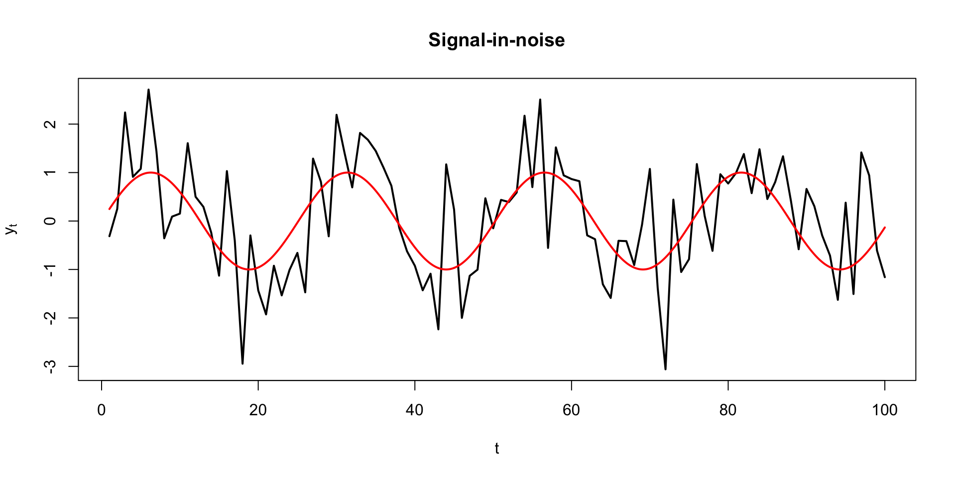
The \(y_t\) we got to see is a corrupted version of some smooth underlying trend or signal \(s_t\) that we wish to extract:

\[ y_t=s_t+\varepsilon_t,\quad \varepsilon_t\iid\N(0\com \sigma^2). \]

Example: stochastic volatility

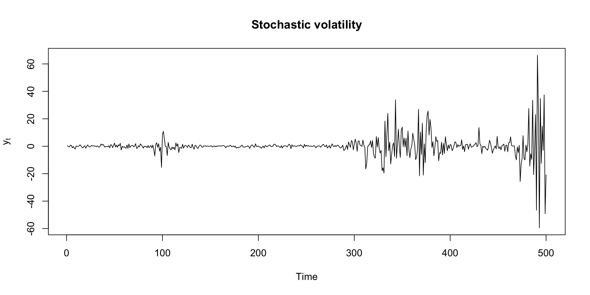
The variance of \(y_t\) is changing over time:

\[ y_t=\mu+\varepsilon_t,\quad \varepsilon_t\indep\N(0\com \sigma_t^2). \]

Example: regime-switching

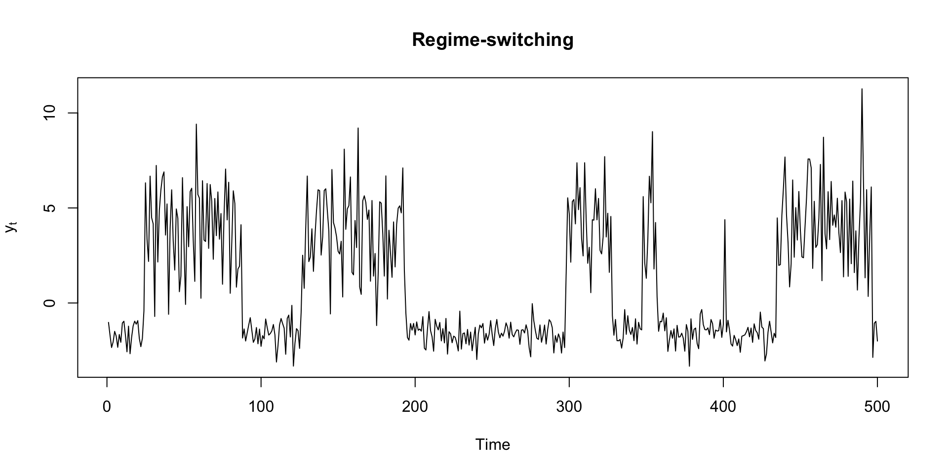
The distribution of \(y_t\) is abruptly switching between a discrete set of options:

\[ y_t \sim \begin{cases} \N(\mu_1\com \sigma^2_1) & \text{if }s_t=1 \\ \N(\mu_2\com \sigma^2_2) & \text{if }s_t=2 \end{cases} \]

Example: time-varying parameter regression

A time-varying linear relationship between response \(y_t\) and predictors \(\Bx_t\):

\[ y_t=\Bx_t^\tr\Bbeta_t+\varepsilon_t. \]

Zoom out

All of those examples have the same basic structure:

An observed time series \(y_t\) depends on an unobserved time series.

Also! All of those models are non-stationary, which we should regard as the rule rather than the exception in time series.

Generic structure

Basic ingredients of all SSMs:

\[ \begin{aligned} \By_t&\sim p(\By_t\given \Bs_t\com \Btheta) && \text{(measurement distribution)}\\ \Bs_t&\sim p(\Bs_t\given \Bs_{t-1}\com \Btheta) && \text{(state transition distribution)}\\ \Bs_0&\sim p(\Bs_0\given \Btheta) && \text{(initial condition)}\\ \Btheta&\sim p(\Btheta). && \text{(parameter prior)} \end{aligned} \]

Graphical structure:

\[ \begin{matrix} \Bs_0 & \rightarrow & \Bs_1 & \rightarrow & \Bs_2 & \rightarrow & \cdots & \rightarrow & \Bs_t & \rightarrow & \cdots \\ & & \downarrow & & \downarrow & & & & \downarrow & & \\ & & \mathbf{y}_1 & & \mathbf{y}_2 & & & & \mathbf{y}_t & & \end{matrix} \]

So the \(\mathbf{y}_t\) are conditionally independent. But this can be relaxed.

Generic goal

Bayesian inference!

\[ \begin{aligned} p(\By_{1:T}\mid \Bs_{1:T}\com\Btheta) &= \prod_{t=1}^T p(\By_t\mid \Bs_t\com\Btheta) && \text{(likelihood)} \\ \\ p(\Bs_{0:T}\mid\Btheta) &= p(\Bs_0\mid\Btheta) \prod_{t=1}^T p(\Bs_t\mid\Bs_{1-t}\com\Btheta) && \text{(state prior)} \\ \\ p(\Bs_{0:T}\com\Btheta\mid\By_{1:T}) &\propto p(\By_{1:T}\mid \Bs_{1:T}\com\Btheta)p(\Bs_{0:T}\mid\Btheta)p(\Btheta) && \text{(posterior)} \end{aligned} \]

We estimate the trend with a posterior mean like \(E(\Bs_{1:T}\mid\By_{1:T})\) or \(E(\Bs_{1:T}\mid\By_{1:T}\com\hat{\Btheta})\).

Dynamic linear model

\[ \begin{aligned} \By_t &= \BF\Bs_t + \Bepsilon_t, && \Bepsilon_t\iid\N_n(\Bzero\com \BV) \\ \Bs_t &= \BG\Bs_{t-1} + \Beta_t, && \Beta_t\iid\N_p(\Bzero\com \BW) \\ & &&\\ \Bs_0&\sim\N_p(\bar{\Bs}_{0|0}\com \BP_0). \end{aligned} \]

  • Special cases: ARMA models, TVP regression, local-level model, etc;
  • The dynamics are governed by system matrices \(\BF\), \(\BV\), \(\BG\), and \(\BW\) which often depend on a lower-dimensional set of parameters \(\Btheta\) that must be estimated.

Local-level model

The simplest non-trivial special case:

\[ \begin{aligned} y_t &= s_t + \varepsilon_t, && \varepsilon_t\iid\N(0\com v) \\ s_t &= s_{t-1} + \eta_t, && \eta_t\iid\N(0\com w) \end{aligned} \]

  • The classic “signal plus noise” model;
  • We set \(\BF=\BG=1\), and the static parameters \(\Btheta=(v\com w)\) control the smoothness and corruption of the signal.

Filtering versus smoothing

Treat \(\Btheta=(v\com w)\) as fixed for now. There are two kinds of signal extraction:

  • \(p(s_t\mid y_{1:t}\com \Btheta)\): “one-sided” estimates of the trend given all data up to the present. This is called filtering;
  • \(p(s_t\mid y_{1:T}\com \Btheta)\): “two-sided”, retrospective estimates of the trend given all data past and present. This is called smoothing.

It’s all posterior inference for the latent variable. The only difference is when the estimate is computed and what data we are conditioning on.

Demo

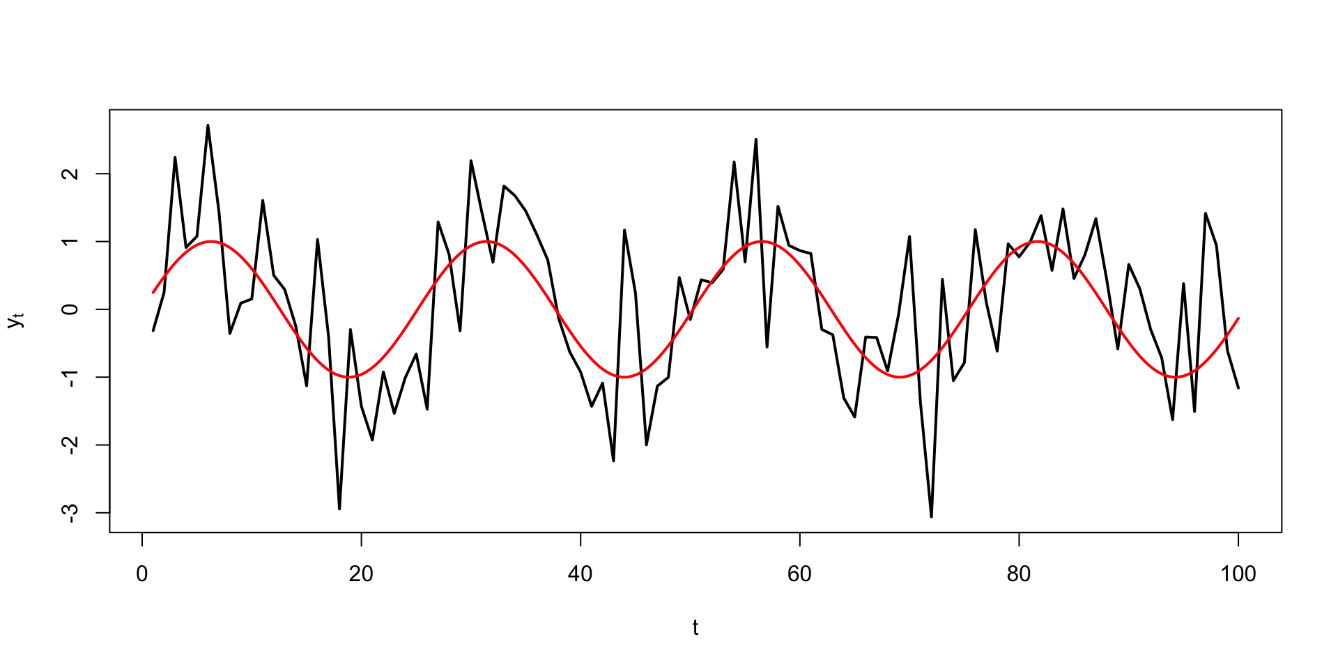
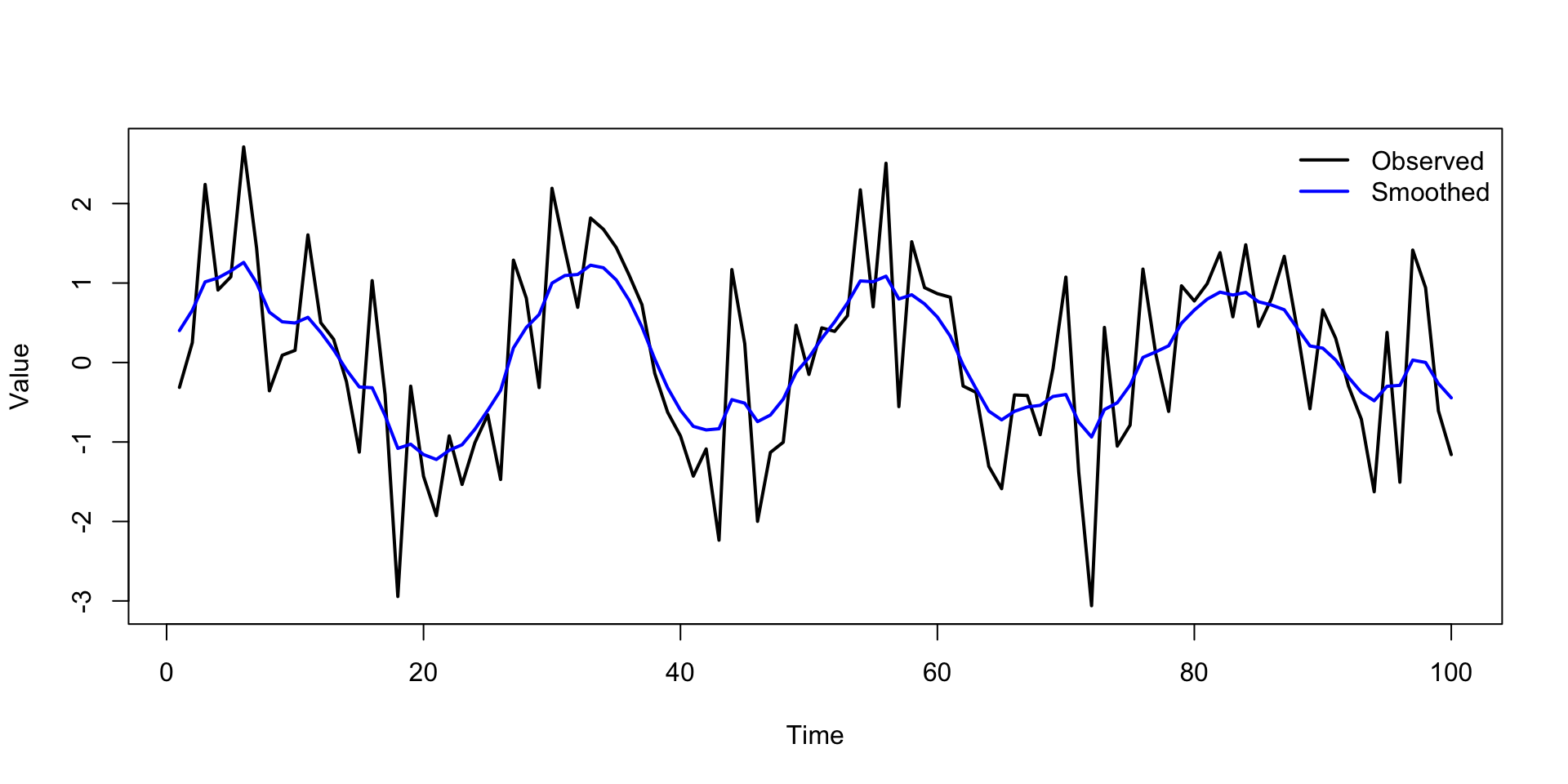
Can we extract the smooth trend from data like these?

\[ y_t\indep\N\left(\sin\left(\frac{t}{4}\right)\com \sigma^2\right). \]

Yes! But the parameters \(\Btheta=(v\com w)\) have a big influence.

The dlm package

  • Created by Duke stats PhD alum Giovanni Petris;
  • Free textbook PDF through Duke library;
  • Accompanying software is well-documented:
library(dlm)

Maximum likelihood

When it comes to estimating \(v\) and \(w\), \(s_{1:T}\) are nuisance parameters that can be fully integrated out using the Kalman filter:

\[ p(y_{1:T}\mid v\com w) = \int p(y_{1:T}\com s_{1:T}\mid v\com w)\,\dd s_{1:T}. \]

This is just a funky multivariate normal! Then we can compute maximum (marginal!) likelihood estimates using numerical optimization:

\[ (\hat{v}\com \hat{w}) = \underset{v\com w}{\arg\max}\,p(y_{1:T}\mid v\com w). \]

Example

Fake data:

set.seed(8675309)
y <- sin((1:T) / 4) + rnorm(T, sd = 1)

MLE in the dlm packages:

# how do the parameters (log-variances) determine the model (local-level)
my_model <- function(x) return(dlmModPoly(order = 1, dV = exp(x[1]), dW = exp(x[2])))

# just passes to the optim function
estimate <- dlmMLE(y = y, parm = c(1, 1), build = my_model)

exp(estimate$par) 
[1] 0.7460911 0.2590706

Empirical Bayes estimate of the trend

This is \(E[s_{1:T}\mid y_{1:T}\com\hat{\Btheta}]\):

Bayesian inference

Put conditionally conjugate priors on the unknown parameters:
\[ \begin{aligned} y_t &= s_t + \varepsilon_t, &&\varepsilon_t\iid\N(0\com v) \\ s_t &=s_{t-1}+\eta_t, &&\eta_t\iid\N(0\com w) \\ v&\sim\text{IG}(a_v\com b_v) \\ w&\sim\text{IG}(a_w\com b_w) . \end{aligned} \]

The full posterior \(p(s_{1:T}\com v\com w\mid y_{1:T})\) is intractable, but we can approximate it with a Gibbs sampler.

Gibbs sampler

To approximate \(p(s_{1:T}\com v\com w\mid y_{1:T})\), cycle through simulating the full conditionals:

  • \(p(v \mid w\com s_{1:T}\com y_{1:T})\): this is inverse gamma;
  • \(p(w \mid v\com s_{1:T}\com y_{1:T})\): this is inverse gamma;
  • \(p(s_{1:T} \mid v\com w \com y_{1:T})\): this is multivariate normal.

The first two steps are very similar to STA 360/402. The last step is the Kalman smoother.

Example

Run the Gibbs sampler:

set.seed(525600)
posterior_draws <- dlmGibbsDIG(
  y,
  dlmModPoly(1),
  shape.y = 1, rate.y = 1, 
  shape.theta = 1, rate.theta = 1, 
  n.sample = 5000,
  progressBar = FALSE
)

Gives you 5,000 draws of \(\{v\com w\com s_{1:T}\}\):

posterior_draws$dV # draws of v

posterior_draws$dW # draws of w

posterior_draws$theta # draws of the states